Understanding Big O Notation
Understanding Big O notation
Understanding Big O is the most fundamental part in understanding the Space and Time complexity concepts that rule in any Data Structure and Algorithms course. Let's put an effort to understand the Big O notation and its limitations in essence.
?Wikipedia’s definition of Big O notation: “Big O notation is a mathematical notation that describes the limiting behaviour of a function when the argument tends towards a particular value or infinity. It is a member of a family of notations invented by Paul Bachmann, Edmund Landau, and others, collectively called Bachmann–Landau notation or asymptotic notation.”
In simple words Big O notation is just an algebraic equation that tells you how complex your code is, i.e., it tells us mathematically that how long an algorithm takes to run (time complexity) or how much memory is used by an algorithm (space complexity).
Why Big O is important?
In the early days of internet era, if you would have talked about the Big O's importance none of us would have bothered as the data that used to be gathered was too less and real time decisions taken by the organisations based upon the data were also too less, all that organisations expected out of the developers is a working code. But of late, where data has become the new fuel for any organisation to grow and sustain, it has become very important to understand the space and time complexity of any algorithm, even a fraction of delay in data processing leads to a heavy business impact these days. So every organisation wants to process and utilise the data quickly and efficiently, here comes the importance of Big O notation as it can express the best, worst, and average-case space and time-complexity of an algorithm.
Reading Big O
To understand how to read Big O notation, we can take a look at a specific example,?O(log n).?
O(log n) is pronounced?“Big O Logarithmic”.
n - input size of the data
log n - function which denotes the complexity of the algorithm.
Summary: O(log n) implies that running time grows in proportion to the logarithm of the input size.
Some basic/most-commonly used Big O notations and their complexity:
O(1) → Constant Time
O(1) means that it takes a constant time to run an algorithm, regardless of the size of the input.
Examples of constant time algorithms include:
Examples of constant space algorithms include:
O(n) → Linear Time
O(n) implies that run time is directly proportional to the input size.
Example of linear time algorithms include:
Example of linear space algorithms include:
O(n2) → Quadratic Time
O(n2) means that run time is directly proportional to the square of input size.
Example of quadratic time algorithms include:
O(log n) → Logarithmic Time
O(log n) means that run time is directly proportional to the log of input size.
领英推荐
Example of logarithmic time algorithms include:
Example of logarithmic space algorithms include:
O(n!) → Factorial Time
O(log n) means that run time is directly proportional to the factorial of input size. This is the most complex algorithm and it's rarely used in real time projects.
Example of logarithmic time algorithms include:
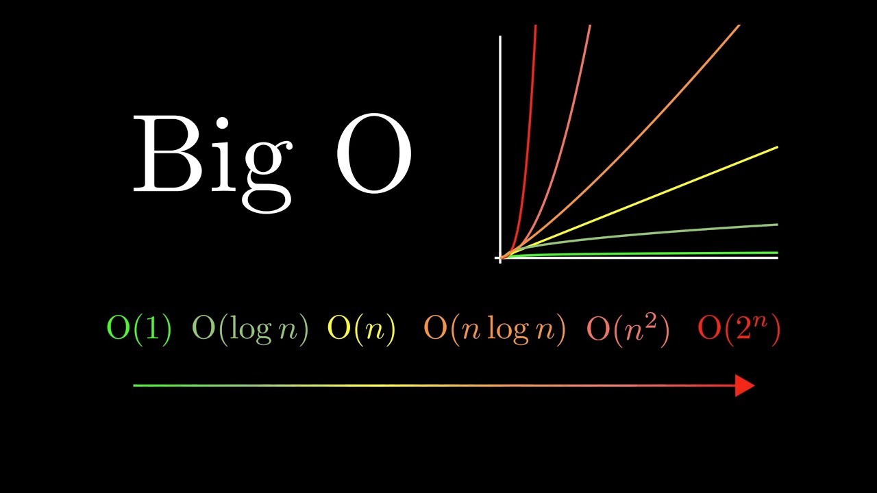
Big O notations' hierarchy and cheat sheet:
One of the best resources to remember the the hierarchy of Big O notations in their increasing order of their complexity is the cheat sheet attached below. You can learn more about space and time Big-O complexities of common algorithms used in Computer Science from the link above.
Basically the entire hierarchy is about exponentiation ranking as listed below:
How to calculate Big O?
While calculating the Big O notation there are some set of rules we should follow so that the calculated notation gives us the holistic idea about how well the given algorithm scales with respect to time and space. So here are the two most basic rules to follow:
Let's calculate Big O for a simple python function shown below
def print_range(n)
    for i in range(100):              step 1
        print(i+1)                    step 2
    print(f'range is {n}')            step 3
    return n                          step 4
f (n) = step 1 + step 2 + step 3 + step 4
f(n) = N + C + C + C
f(n) = N+3C
Following the rule number 1, we need not consider constant parts of the algorithm like step 2, step 3, step 4 whose execution is not dependent on the size input. 'step 1' is the only part where the execution of 'for' loop depends on the size (N) of the input. Also second rule makes it clear that we should drop the non dominant terms, in this is 3C. Hence the final equation reduces to f(n) = N.
Big O = O (f(n)) = O(N)
Hence the above algorithm grows linearly in proportion to the size of the input.
Conclusion
Even though the Big O notation gives us the fair amount of idea about the given algorithm's space and time complexity, in real life the decision regarding implementation of an algorithm will taken by considering other computational capacities like RAM, processors, and size of the input data. Hence there will be trade offs involved among the computation capacity, time required to finish the task, size of the input etc.
Now you might be wondering, if the decision regarding implementation of an algorithm is not solely dependent on Big O's complexity, then what's the use of putting efforts to understand this complex thing. But, having an in depth understanding of the Big O concept will help you to design better algorithms and it's like alphabet of programming.
This is all about Big O, will talk about trade-offs while choosing the sorting algorithms in my next article, which is more like an applied Big O thing.
This is my first LinkedIn article and I am aficionado of Apache products. I will write more about them and other data related topics in the coming days.
Happy Learning...!