Optimizing Machine Learning Models with Bayesian Optimization: A Deep Dive into Gaussian Processes and Hyperparameter Tuning

Introduction

Hyperparameter tuning is one of the most critical aspects of training a machine learning model. Properly tuned hyperparameters can make the difference between a mediocre model and one that achieves state-of-the-art performance. Traditionally, grid search and random search have been the go-to methods for hyperparameter optimization. However, these methods can be computationally expensive and inefficient, especially when dealing with large search spaces.

This is where Bayesian Optimization comes into play, offering a more efficient approach to hyperparameter tuning by leveraging probabilistic models to explore the search space intelligently. In this article, we’ll explore Bayesian Optimization, its underlying mechanism using Gaussian Processes, and how we applied it to optimize a machine learning model on the Breast Cancer dataset.

What is a Gaussian Process?

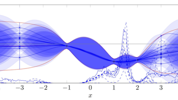
A Gaussian Process (GP) is a powerful non-parametric model used for making predictions about uncertain functions. At its core, a GP is a collection of random variables, any finite number of which have a joint Gaussian distribution. GPs are widely used in regression tasks due to their flexibility and ability to provide uncertainty estimates.

In a machine learning context, a GP defines a distribution over functions, which can be updated as more data is observed. This makes GPs particularly well-suited for Bayesian Optimization, where the goal is to make informed decisions about which hyperparameters to try next, based on past observations.

Mathematical Formulation:

Given a set of input points X={x1,x2,...,xn} and their corresponding function values y={y1,y2,...,yn}, a Gaussian Process assumes that the joint distribution of the function values is Gaussian:

y～N(0,K(X,X))

where K(X,X)K(X, X)K(X,X) is the covariance matrix defined by a kernel function. The kernel function encodes our assumptions about the function we are modeling, such as smoothness and periodicity.

What is Bayesian Optimization?

Bayesian Optimization (BO) is an approach to optimize objective functions that are expensive to evaluate. It is particularly useful when we do not have a closed-form expression for the objective function and when evaluations of the function are costly.

BO works by constructing a probabilistic model of the objective function, typically using a Gaussian Process, and then using this model to make decisions about where to evaluate the function next. The process involves the following steps:

1. Construct a surrogate model: A Gaussian Process is typically used to model the objective function.
2. Choose a point to evaluate: An acquisition function (e.g., Expected Improvement) is used to select the next point to evaluate, balancing exploration and exploitation.
3. Update the model: After evaluating the function at the selected point, the model is updated with the new data.
4. Repeat: This process is repeated until a stopping criterion is met (e.g., a maximum number of iterations or a satisfactory solution is found).

Bayesian Optimization is particularly powerful because it reduces the number of evaluations needed to find an optimal solution, making it ideal for hyperparameter tuning in machine learning.

The Chosen Model and Hyperparameters

For this task, I chose to optimize a simple neural network model on the Breast Cancer dataset from sklearn’s datasets. The model is a Sequential model built using Keras, with one hidden layer followed by a dropout layer and an output layer for binary classification.

Here's how the model is structured in code:

from tensorflow.keras.models import Sequential
from tensorflow.keras.layers import Dense, Dropout
from tensorflow.keras.regularizers import l2

def build_model(learning_rate, units, dropout_rate, l2_reg):
    model = Sequential()
    model.add(Dense(units=units, activation='relu', input_shape=(X_train.shape[1],),
                    kernel_regularizer=l2(l2_reg)))
    model.add(Dropout(rate=dropout_rate))
    model.add(Dense(units=1, activation='sigmoid'))
    return model
        

The hyperparameters I focused on optimizing were:

1. Learning Rate: Controls how much to adjust the model's weights with respect to the loss gradient.
2. Number of Units in the Hidden Layer: The number of neurons in the hidden layer, which affects the model's capacity.
3. Dropout Rate: Helps prevent overfitting by randomly setting a fraction of input units to zero at each update during training.
4. L2 Regularization Weight: Adds a penalty to the loss function for large weights, encouraging the model to find smaller weights.
5. Batch Size: The number of samples processed before the model is updated.

These hyperparameters were chosen because they are crucial to the performance of the neural network, and they interact in complex ways. Tuning them effectively can lead to significant improvements in model accuracy and generalization.

Satisficing Metric and Early Stopping

For this optimization task, I chose validation accuracy as the satisficing metric. The goal was to maximize this metric, which directly corresponds to the model's ability to generalize to unseen data. Early stopping was used during training to prevent overfitting and ensure that the best model was saved based on the highest validation accuracy achieved.

Implementing Bayesian Optimization with GPyOpt

To optimize the model, I used GPyOpt, a popular library for Bayesian Optimization in Python. Below is the core code snippet for the optimization process:

import GPyOpt

def model_score(params):
    learning_rate = float(params[:, 0])
    units = int(params[:, 1])
    dropout_rate = float(params[:, 2])
    l2_reg = float(params[:, 3])
    batch_size = int(params[:, 4])

    model = build_model(learning_rate, units, dropout_rate, l2_reg)
    
    checkpoint_path = f'checkpoint_lr_{learning_rate}_units_{units}_dropout_{dropout_rate}_l2_{l2_reg}_batch_{batch_size}.h5'
    callbacks = [
        EarlyStopping(monitor='val_accuracy', patience=5, restore_best_weights=True),
        ModelCheckpoint(checkpoint_path, monitor='val_accuracy', save_best_only=True, verbose=1)
    ]
    
    history = model.fit(X_train, y_train,
                        validation_data=(X_val, y_val),
                        batch_size=batch_size,
                        epochs=50,
                        callbacks=callbacks,
                        verbose=0)
    
    val_acc = np.max(history.history['val_accuracy'])
    return -val_acc

# Define the bounds of the hyperparameters
bounds = [
    {'name': 'learning_rate', 'type': 'continuous', 'domain': (1e-5, 1e-1)},
    {'name': 'units', 'type': 'discrete', 'domain': (16, 32, 64, 128, 256)},
    {'name': 'dropout_rate', 'type': 'continuous', 'domain': (0.0, 0.5)},
    {'name': 'l2_reg', 'type': 'continuous', 'domain': (1e-6, 1e-2)},
    {'name': 'batch_size', 'type': 'discrete', 'domain': (16, 32, 64, 128)}
]

# Perform Bayesian Optimization
optimizer = GPyOpt.methods.BayesianOptimization(f=model_score, domain=bounds)
optimizer.run_optimization(max_iter=30)
        

Visualizing the Optimization Process

Here’s a plot showing the convergence of the optimization process, highlighting how the validation accuracy improved over iterations:

This plot underscores the efficiency of Bayesian Optimization in finding the best hyperparameter configuration in fewer iterations compared to traditional search methods.

Conclusions from the Optimization

The optimization process effectively identified a set of hyperparameters that improved the model's validation accuracy. The use of Bayesian Optimization reduced the number of evaluations needed compared to traditional methods like grid search, and the final model demonstrated better generalization performance on the validation set.

The key takeaway is that Bayesian Optimization, guided by a Gaussian Process, is a powerful tool for hyperparameter tuning. It not only saves computational resources but also leads to better-performing models in fewer iterations.

Final Thoughts

Hyperparameter optimization is a critical step in building robust machine learning models. By leveraging Bayesian Optimization with Gaussian Processes, we can significantly streamline this process, leading to better models with less computational effort. The approach outlined in this article can be applied to various machine learning models and tasks, making it a versatile tool in any data scientist's toolkit.

If you're interested in more technical insights and implementations, connect with me on LinkedIn.

Let's continue exploring the fascinating world of machine learning together!

References:

• Gaussian Processes for Machine Learning
• Bayesian Optimization for Hyperparameter Tuning
• Keras Documentation
• Max Planck Institute for Intelligent Systems