Mastering Software Testing: Unlocking the Power of Metrics for Effective Process Management.
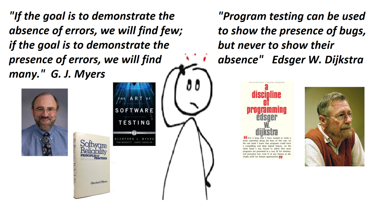
The image I composed to introduce this article shows two people belonging to that group of computer scientists who made the history of computer science.
I chose them because I believe their statements sum up the entire discipline of software testing.
Everything I will write in these five or six articles dedicated to software testing can be derived from these two sentences. After this necessary preamble to the article, let's continue with the third stage of our journey (4.), (5.).
The topic of this article is to find the answer to fundamental questions in software testing like: When do we stop testing? and How good then is the software? We will delve into metrics, specifically the quality metrics that should drive the software testing process.
However, let's kick off the article with a brief subject that I should have covered in the first stage of this journey but realized I touched upon too superficially. It is about the need to engage testers from the beginning so to prevent defects because "Prevention is Cheaper Than Cure" (2.).
I want to emphasize the need for testers to be involved from the beginning of a project's life cycle so they can understand exactly what they are testing and can work with other stakeholders to create testable requirements.
"Defect prevention" can help detect and avoid errors before they propagate to later development phases. Defect prevention is most effective during the requirements phase, when the impact of a change required to fix a defect is low: the only modifications will be to requirements documentation and possibly to the testing plan, also being developed during this phase. If testers are involved from the beginning of the development life cycle, they can help recognize omissions, discrepancies, ambiguities, and other problems that may affect the project requirements' testability, correctness, and other qualities.
A requirement can be considered testable if it is possible to design a procedure in which the functionality being tested can be executed, the expected output is known, and the output can be programmatically or visually verified.
Testers need a solid understanding of the product so they can design better and more complete test plans, procedures, and cases. Early test-team involvement can eliminate confusion about functional behavior later in the project life cycle. In addition, early involvement allows the test-team to learn over time which aspects of the application are the most critical to the end user and which are the highest-risk elements. This knowledge enables testers to focus on the most important parts of the application first, avoiding over-testing rarely used areas and under-testing the more important ones.
The earlier in the life cycle a defect is discovered, the cheaper it will be to fix it. The following table shows the relative cost to fix a defect depending on the life-cycle stage in which it is discovered.
Starting testers early essentially means having them already working on the requirements.
It is important that guidelines for requirements development and documentation are defined at the beginning of the project. Use cases are a way to document functional requirements and can lead to more in-depth system designs and testing procedures.
In addition to functional requirements, it is important to also consider Non-functional requirements, such as performance and security, early in the process: they can determine technology choices and risk areas. Non-functional requirements do not give the system any specific function, but rather constrain how the system will perform a certain function. Functional requirements should be specified along with associated non-functional requirements.
Following is a checklist that can be used by testers during the requirements phase to verify the quality of the requirements. Using this checklist is the first step to identify requirements-related defects as early as possible, so that they do not propagate to subsequent phases, where it would be more difficult and expensive to find and correct them (3.).
As soon as a single requirement is available for review, it is possible to start testing that requirement for the above-mentioned characteristics. Catching requirements defects as soon as they can be identified will prevent incorrect requirements from being incorporated into design and implementation, where they will be more difficult and expensive to find and fix.
Writing these considerations I became convinced that we should dedicate an entire stage of this journey to a study on "requirements" and "use cases". I will do it in one of the next articles in this series on software testing.
Now let's move on to the main topic of this article, which is the importance of using metrics in the software testing process (1.).
But why is it so important to have a measurement? Well I'll try answering the following question.
Would you hire a bricklayer who didn't have a plumb line and a bubble level? Probably not, because the bricklayer who does not use a plumb line and a bubble level will probably not be able to do a satisfactory result. Most people recognize readily that measuring tools are necessary for a bricklayer to make sure that the floors are level and the walls plumb.
So why should we buy software to do important work if it was developed and validated by people who don't use any kind of measurement?
In this article we define the fundamental testing metrics that can be used to answer the following questions.
Time, cost, tests, bugs are some of the fundamental metrics specific to software testing. Derived test metrics can be made by combining these fundamental metrics. The problem is that only time and cost are clearly defined by standard units. For tests and bugs we need to define new specific unit measures.
So let's start with time and cost.
The question "How big is it?" is usually answered in terms of how long it will take and how much it will cost. These are the two most common attributes of it. We would normally estimate answers to these questions during the planning stages of the project. These estimates are critical in sizing the test effort and negotiating for resources and budget.
Units of time are used in several test metrics, for example, the time required to run a test. This measurement is absolutely required to estimate how long a test effort will need in order to perform the tests planned. It is one of the fundamental metrics used in the test inventory and the sizing estimate for the test effort.
The cost of testing usually includes mainly the cost of the testers' salaries. It may be quantified in terms of the cost to run a test or the entire Tests Inventory.
Therefore calculating the cost of testing is simple.
But how can we quantify the cost of not executing the testing phase? We can assert that the cost of not taking the test is proportionally higher to the potential number and severity of bugs that would have been identified and resolved if the testing phase had been executed.
We can certainly claim that finding bugs is the main purpose of testing.
Bugs are often debated because there is no absolute standard in place for measuring them. Let's see the main bugs metrics:
Severity is a fundamental measure of a bug or a failure. Many ranking schemes exist for defining severity. Because there is no set standard for establishing bug severity, the magnitude of the severity of a bug is often open to debate. We have already seen this aspect of bugs in the first article of this series (4.)
For instance, in a severity classification, defects might fall into the following categories:
The "Number of Bugs Found" is another metric about bugs.
It is useful to split this metric in two values:
Remember that this is a rather weak measure if we do not integrate it with the severity of the detected bugs. But improved with this information it becomes an important metric in establishing an answer to the question "Was the test effort worth it?"
Another measure about bugs is the "Number of Bugs Found by Testers per Hour".
This is a most useful derived metric both for measuring the cost of testing and for assessing the stability of the system. Consider the tables below. The following statistics are taken from a case study. These statistics are taken from a five-week test effort conducted by testers on new code. These statistics are a good example of a constructive way to combine bug data, like the bug fix rate and the cost of finding bugs, to report bug information.
Notice that the cost of reporting and tracking bugs is normally higher than the cost of finding bugs in the early part of the test effort. This situation changes as the bug find rate drops, while the cost to report a bug remains fairly static throughout the test effort.
By week 4, the number of bugs being found per hour has dropped significantly. It should drop as the end of the test effort is approached. However, the cost to find each successive bug rises, since testers must look longer to find a bug, but they are still paid by the hour.
These tables are helpful in explaining the cost of testing.
Still on the metrics about bags we have the "Bug Density per Unit" metric. This metric answers the following question "Where Are the Bugs Being Found?"
Figure below shows the bug concentrations in four modules of a system during the system test phase. A graph of this type is one of the simplest and most efficient tools for determining where to concentrate development and test resources in a project. It is also an excellent information for developers to guide their refactoring work. Bug densities should be monitored throughout the test effort. The graph below shows both the number of bugs and the severity of those bugs in the four modules.
This type of chart is one of the most useful tools testers have for measuring code reliability
Also very important is the metric "Bug Composition" which allows us to answer the question "How Many of the Bugs Are Serious?".
As we have just said, there are various classes of bugs. Some of them can be fixed easily, and some of them cannot. The most troublesome bugs are the ones that cannot be easily reproduced and recur at random intervals. Software
bugs are measured by quantity and by relative severity. If a significant percentage of the bugs being found in testing are serious, then there is a definite risk that the users will also find serious bugs in the shipped product.
Figure below shows the graphical representation of the bugs found.
The Severity 1 bugs reported represent 38 percent of all bugs found. That means that over a third of all the bugs in the product are serious. Simply put, the probability is that one of every three bugs the user finds in the product will be serious.
Again, to answer the question "How Many of the Bugs That Were Found Were Fixed?" we have the the "Bug Fix Rate" measure.
Bug fix rate = (BugsFixedDuringTest / BugsFoundDuringTest)*100
The figure below shows an example of cumulative errors found and errors fixed curves for a case study. The gap between the two curves at the end of the scale is the bugs that were not fixed.
Some bugs could be classified as "hard to reproduce." A study of production problems showed that over the 50% of the problems that occurred in production had been detected during the system test. However, because the test effort had not been able to reproduce these problems or isolate the underlying errors, the bugs had migrated into production with the system due to the rush to delivery the product. The risk of not delivering the product on time sometimes wins the risk of leaving bugs that cannot be easily reproduced or are not well understood. If there is no estimation of the risk of releasing these bugs, management does not have enough information to make a well-informed decision. The pressure to delivery on time becomes the overriding factor.
Well now that we have seen the bug metrics we can move on to the topic of Residual Bug Estimation. We could finally answer the question "How many bugs are still hidden in software under development?". It is extremely useful to know when to stop testing, or to estimate how many bugs will be left in the program if we stop testing “now”.
The model we see is the Goel-Okumoto model which requires bug tracking (detection time) and effort tracking (man-hours).
The Goel-Okumoto model is used to predict the number of residual bugs remaining in software after a certain amount of testing or debugging effort has been expended. This model is focused on estimating the number of residual defects yet to be discovered in a software system.
The Goel-Okumoto model is based on the assumption that the rate at which faults are detected decreases as testing progresses. It's a dynamic model that predicts the number of residual bugs over time and is widely used in software reliability engineering. The fundamental equation of the Goel-Okumoto model is:
领英推荐
where B(t) is the total number of bugs found at time t, while a and b are two constants to be found, which represent the total number of bugs in the product and the bug detection rate. Look at the chart below.
This model helps to make predictions about the number of remaining undiscovered bugs, assisting software development teams in planning and estimating the resources needed for future testing and debugging activities. However, like many models in the field of software engineering, the accuracy of predictions heavily relies on the quality of the data used to estimate the model's parameters and the assumptions made in its application.
To draw the graph, we need to know how many bugs per man/hour have been found: t is not calendar time! We may need to normalize incoming data.
Below we see two real cases that I handled a few years ago. The first concerns the software of an embedded treadmill platform for cardiovascular exercise with the integrated TV for entertainment and the Web for internet browsing (around 250,000 lines of source code, around 80 primary use-cases, Object Oriented design paradigm).
The second example is a NFC reader of a "mifare" tag used to log-in the customer to the treadmill. Besides it reads the programmed exercise and automatically set up the loads (speed and incline) in the equipment and then saves the customer's results at the end of the exercise(around 5,000 lines of source code, about 4 primary use-cases, procedural design paradigm).
In the past when I managed a software quality assurance team I used Okumoto's model a lot. I have regulated its use in a company operating procedure on software quality. In particular, the analysis of the Okumoto graph was part of the criteria for completing the test. We will look at this criteria in the final part of this article, after we have seen the TPE metric.
Let's now look at the metrics to measure the Test Effort and Test Effectiveness.
Let's start with a metric that gives us an answer to follow question "How Good Were the Tests?"
There is a simple metric to evaluate the goodness (intended as test case coverage) of a test plan. This metric is called "Test Case Effectiveness" (TCE).
We define Np, Nr, Nt and TCE as follows:
Np = number of bugs with planned tests.
Nr = number of bugs found with random tests.
Nt = Np + Nr
TCE = Np / Nt
TCE represents the ratio of the number of bugs found with planned tests (Np) to the total number of bugs found, including those uncovered by random tests (Nr), resulting in Nt where Nt = Np + Nr. Naturally, TCE falls within the range of 0 to 1, with the objective of having TCE as close to 1 as possible, indicating that most bugs have been detected through planned tests.
Please note that it is essential that the random test is performed on features that have already been tested with the planned testing.
Assuming we have a way to measure “how much use cases or code did the tests cover” (we’ll see it soon), we split TCE and coverage using a threshold (e.g. 0.75) and then we have four sectors.
The good test plan is the one that falls in sector "High TCE - High Coverage".
But, we still left one question un-answered : "How Much of It Was Tested?"
To answer this question we need a measure for "Test Coverage".
A simple way is to refer to the Test Inventory (the set of all test cases) of our planned tests which have been designed starting from both the system's use cases and the non-functional requirements (as we have already seen in the first part of this article).
System test coverage is then a measure of how many of the tests in a our inventory were exercised.
System Test Coverage = (Test Executed / Total Test Inventory)* 100
The value of this test coverage metric depends on the quality and completeness of the test inventory.
In some situations, however, this measure of coverage based on test inventory is not sufficient. For example, software in the equipment for medical market may require a specific certification on the test execution that demonstrates the coverage of the instructions or paths
Testers, with the assistance of developers if they are not proficient in code reading, can assess code coverage during execution. This means tracking traversed lines in the code. It serves two essential purposes: to provide a coverage percentage and to highlights which statements have not been covered.
Branch and path testing, within the white box context, introduce additional complexity. Testers must differentiate between statements, branches, and paths in the code. A single statement may be reached through different branches, while a single branch may be part of various paths. Branches typically correspond to decision points in the code's control flow.
The two images below clarify the difference between statements, branches and paths:
Ideally, testers should test each branch, not just each statement, to ensure comprehensive coverage. However, testing each path is a more demanding and exhaustive task, often requiring careful consideration of various scenarios and logic flow within the code.
Now that we have found the metrics that allow us to measure the Coverage and Effectiveness of our test inventory and that we have learned to use a Residual Bug Estimation model we can finally establish an empirical criteria in order to declare the test phase completed.
Indeed, to be precise, we will see a criteria for considering the test phase of the testers concluded because as a matter of facts the testing never ends, it simply passes from the testers group to the customer.
The test completion criteria that I have used over the many years that I managed the software quality assurance team consists of the following four rules:
Depending on the software project under test the limits in each of the four rules may be revised. For example a limit of 2% from OKUMOTO's ideal curve might be acceptable for case where there have been many software changes during the testing phase or even a lower TCE when overdoing the random tests.
The power of this criteria is in the simultaneous verification of different metrics that measure different aspects of the software testing process.
That's all for this third stage of our software testing journey, in the next article we will talk about Regression Testing and Test Automation.
See you on the next episode
I remind you my newsletter?"Sw Design & Clean Architecture"? :?https://lnkd.in/eUzYBuEX?where you can find my previous articles and where you can register, if you have not already done, so you will be notified when I publish new articles.
Thanks for reading my article, and I hope you have found the topic useful,
Feel free to leave any feedback.
Your feedback is very appreciated.
Thanks again.
Stefano
References:
1.?Marnie L. Hutcheson, “Software Testing Fundamentals: Methods and Metrics”, John Wiley & Sons (2003).
2.?Elfriede Dustin, “Effective Software Testing: 50 Specific Ways to Improve Your Testing”, Addison Wesley (2002).
3. Dean Leffingwell, Don Widrig "Managing Software Requirements", Second edition, Addison Wesley (2003)
4.?S. Santilli: "https://www.dhirubhai.net/pulse/mastering-art-software-testing-guide-testers-stefano-santilli-fpomf/".?
5.?S. Santilli: "https://www.dhirubhai.net/pulse/unveiling-effectiveness-black-box-testing-software-quality-santilli-nrv8f".?