Fast & explainable clustering with CLASSIX: Quick start

In today's post, I demonstrate the CLASSIX clustering method using its Python implementation. A discussion of the inner workings of this method will be part of another post. For now, it suffices to know that CLASSIX is primarily a distance-based clustering method. This means: the dominating quantity that determines whether two data points become part of the same cluster is simply their distance. CLASSIX also shares some properties with density-based clustering methods like DBSCAN, but this is not relevant for the below demonstration.

Installation

We first need to install CLASSIX via PIP:

pip install classixclustering        

The GitHub repository is https://github.com/nla-group/classix

Method parameters

CLASSIX is controlled by two parameters, radius and minPts (optional). The radius parameter determines the granularity of the clusters. When radius is decreased, the number of clusters generally increases. We recommend starting with radius=1 and decreasing this value successively until the number of clusters is only slightly larger than expected. The minPts parameter can then be used to remove tiny clusters with only a small number of data points. The default value is minPts=1, i.e., a cluster should include at least one data point.

Usage

The below Python code generates a synthetic dataset of 20,000 points, forming five Gaussian blobs in 5-dimensional space. It then calls CLASSIX and prints some statistics about the clustering.

import classix
from time import time
from sklearn.datasets import make_blobs
from sklearn.metrics import adjusted_rand_score as ari
from sklearn.metrics import adjusted_mutual_info_score as ami

# generate data and ground-truth labels y
data, y = make_blobs(n_samples=int(2e5),centers=5,n_features=5,random_state=42)

# run CLASSIX
clx = classix.CLASSIX(radius=0.17, verbose=0)
st = time()
clx.fit(data)
et = time()

print("CLASSIX  version:", classix.__version__)
print("adjusted Rand index (ARI): ", ari(clx.labels_, y))
print("adjusted mutual info (AMI):", ami(clx.labels_, y))
print("CLASSIX runtime in seconds:", et - st)        

CLASSIX version: 1.0.5 
adjusted Rand index (ARI):  1.0 
adjusted mutual info (AMI): 1.0 
CLASSIX runtime in seconds: 0.702845573425293        

This took just under a second. The ARI and AMI numbers are measures for the quality of the clustering, which in this case is perfect.

The explain functionality

CLASSIX is an explainable clustering method which provides justifications for the computed clusters. We can use the .explain() method to get a first overview of the clusters:

clx.explain(plot=True)        

Note that the original data lives in 5-dimensional space but, for the plot, CLASSIX projects the data onto the first two principal axes. It looks as if two of the clusters are merged, but they are actually well separated in 5D.

CLASSIX follows up with textual information about the clustering:

CLASSIX clustered 200000 data points with 5 features.
The radius parameter was set to 0.17 and minPts was set to 1.
As the provided data was auto-scaled by a factor of 1/11.98,
points within a radius R=0.17*11.98=2.04 were grouped together.
In total, 12280544 distances were computed (61.4 per data point).
This resulted in 1162 groups, each with a unique group center.
These 1162 groups were subsequently merged into 5 clusters. 

To explain the clustering of individual data points, use
.explain(index1) or .explain(index1,index2) with data indices.        

I will discuss this output in more detail in another post. However, we can already follow the last hint and call .explain() with the indices of two data points. In this case, CLASSIX will provide an explanation for why the points ended up in the same cluster, or not. Let's try it out:

clx.explain(270,2794,plot=True)        

Data point 270 is in group 630.
Data point 2794 is in group 507.
Both groups were merged into cluster #2. 

The two groups are connected via groups
 630 <-> 526 <-> 507.

Here is a list of connected data points with
their global data indices and group numbers:

  Index  Group
   270    630
177067    630
 77248    526
 80149    507
  2794    507         

CLASSIX explains that there is a path of data points (indices 270, 177067, …, 2794) that connects the two data points 270 and 2794. The distance between the points on the path is less than radius (after data scaling), and this is why they are all in the same cluster #2. In other words, we can connect all these data points making only small steps and without leaving the cluster.

Performance comparison

At this point you may wonder, how does CLASSIX compare to other clustering methods? In particular, the Gaussian blob dataset is the perfect use case for k-means clustering (provided the number of clusters is known). And of course, there are many many other popular methods like DBSCAN, HDBSCAN, Quickshift, spectral clustering, etc. which one could use.

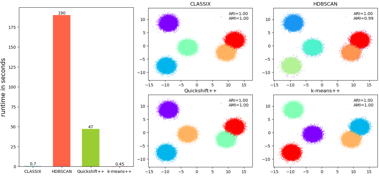
Here are the results of a performance comparison which is part of CLASSIX's demo collection (https://github.com/nla-group/classix/blob/master/demos/Performance_test_Gaussian_blobs.ipynb)

The CLASSIX paper compares many more algorithms on various datasets. The hyperparameters of each method have been tuned by grid search. The k-means++ method has been provided with the ground-truth of k=5 clusters. Should you find a set of hyperparameters that improves a method significantly, please let us know in the comments and we will update this benchmark.

The overall conclusion is clear. In terms of runtime, k-means is the fastest method for this dataset (0.45 seconds), closely followed by CLASSIX (0.7 seconds). HDBSCAN (180 seconds) and Quickshift++ (47 seconds) are significantly slower. All methods compute (almost) perfect clusterings for this dataset in terms of ARI/AMI.

Next week we will look at clustering a real-world dataset with more than 5 million data points. In the meantime, should you have any questions or comments, or even have some interesting datasets to try out, please let me know in the comments.