Face Detection using Haar Cascade Algorithm
Face detection is a common need nowadays, with many applications and devices using it. Many algorithms have been built to achieve this purpose. One such algorithm is the Haar Cascade algorithm. The algorithm was discussed back in 2001 by Viola and Jones and was published under the paper named “Rapid Object Detection using a Boosted Cascade of Simple Features”. Though many years have passed, this algorithm still has broader applications in computer vision and image processing. This technique can be implemented in images as well as in real-time video to detect the faces and eyes.
In this article, I will try to discuss the working of algorithm in a simplified manner, and later, I will implement this technique via a pre-trained model using OpenCV and Python.
The article can be divided into three parts basically:
I will discuss all the part one by one:
Part-1: Integral Image
The algorithm was trained on 4916 hands labeled images and 9544 non-face images. To train the images, there was a need to extract features from the images. It could have worked on pixels directly instead of using features. This is due to the fact that feature-based systems are substantially faster than pixel-based systems. And it becomes very useful when there are number of pixels to be scanned. Before diving into integral image part, first let’s understand features to identify the faces.
The three main features that were used:
Let’s discuss it for the edge features. Edge features are responsible for finding the horizontal and vertical lines in the images. Here, the difference between the sum of pixels in within two rectangular regions determines the value of a two-rectangle feature (shown in figure-1). It means to obtain a feature value, first we find the sum of all pixels inside the white rectangle and then find the sum of all pixels inside the black rectangle and then subtract the mean of the sum of pixles from the white rectangle to the mean of the sum of pixels of the black rectangle.
Let’s compute the sum for figure 4-b) for both lighter region pixels and darker region pixels.
Lighter region → sum([0,0.1,0.3,0.1,0.1,0.2,0.2,0.2]) = 1.2
Darker region → sum([0.8,1,0.7,0.8,0.8,0.8,0.8,0.8]) = 6.5
Mean of lighter region → 1.2/8 = 0.15
Mean of darker region → 6.5/8 = 0.8125
Differences of mean of lighter and darker region = 0.8125–0.15 = 0.6625
So, we got 0.6625 as the difference. The closer the result is to 1, better a feature. We can define a threshold to classify whether this feature passed or whether to discard. It could be 0.6 or 0.7 or any value. Suppose the threshold was set for 0.6; hence it passed, and we can say that edge detected.
In the case of three rectangle features, the sum of pixels of two outside rectangles is computed and then subtracted from the sum of pixels of the rectangle present inside. Three set of rectangular features, as its structure suggests, describe whether there is a lighter region surrounded by a darker region.
And in the case of four rectangle features, as the structure suggests, we find the sum of pixels of the diagonally darker region and then subtract it from the sum of pixels of the lighter region. This set of rectangular features is responsible for detecting pixel intensity changes across diagonals.
Like the convolutional filter of CNN, haar features traverse from top left to bottom right, step by step.
We have shown above that how the feature calculation is done. But doing this calculation for the entire image would lead to a large amount of time and hence is computationally expensive. With 24 x 24 resolution of the detector, the overall image contains a set of features of more than 180,000, there needs to have a better approach.
So, the authors come up with the concept of Integral Image. It is also known by the summed area table. Each pixel in an Integral Image is the sum of all pixels to its left and above in the Original Image. It is also known by the summed area table.
Mathematcially:
Creating the Integral image of the image is very simple and independent of size. We can do it in raster scan fashion in a single scan of image. The sample of integral image is shown below:
In the above, notice that 3490 (fig -5b) represents the sum of all yellow portioned numbers.
Now consider a situation,if we want to find the brightness of pixel 3490, denoted in yellow below, this is how we will calculate.
We will calculate this by subtracting the pixels with value 1249 and 1137 (denoted by pink box in figure 6-a) and adding 417 (denoted by sky-blue box in figure 6-b).
For better understanding, let’s go deeper into this:
In the image pixel 1137, which was represented using sky blue in figure 6-b, is represented by a rectangle sky blue (for easy identification), and similarly pixel 1249 is represented by pink color rectangle in figure 6-a. Notice that common rectangle containing numbers, (98,110,99,110) has been subtracted twice. So it needs to be added , which leads us to formula:
In internal image.
Sum = A — B — C + D
Where A = Yellow box in figure 6b
B = Sky Blue box in figure 6b
C = Pink box in figure 6b
D = Green box in figure 6b
Now let’s see how does Haars value get calculated in integrated image. Let’s visualize it through the image.
As we know that formula for calculating haar cascade is given by:
= Sum of pixels in white region — sum of pixels in dark region
= (2061–329–584+98 ) — (3490–576–2061+329)
= 64
In the above picture, logic which we have discussed earlier is followed. To compute white pixels where total sum is 2061, pixles 584 and 329 has to be subtracted, and 98 which has been subtracted twice, needs to be added. Same logic needs to be followed for black region.
Here above all the red color boxes denotes , pixels that needs to be subtracted and green color box, denotes pixels need to be added. In this way complexity reduces by a great amount.
Part-2: Adaboost
There were over 180,000 rectangles features associated with the each image sub-window, and this number was significantly larger than number of pixels. Despite the fact that each characteristic can be computed quickly, computing the entire set was prohibitively expensive. So, a feature slection technique was needed. And basically this was a classification problem, as we had the features and the training set, any machine learning algorithm could be applied. The authors of the algorithm decided to go with Adaboost, to select a small subset of features and train the classifier.
After experimenting, it was found out that very small number of these features can be combined to form an effective classifier. So, to achieve this goal, weak learning algorithm was designed to single rectangle feature, which best separates the positive and negative examples. The weak learner chooses the best threshold function for each feature so that the least amount of examples are misclassified.
In each round of boosting, Adaboost algorithm selects one feature from the possible features of 180,000.
Initial rectangle features selected by Adaboost were meaningful and could be easily interpreted. The whole idea of feature selection was based on two properties: Region of eyes are often darker than the region of nose and cheeks. So this feature compares the difference in intensity between the region of eyes and region of cheeks. And the second feature was based on property that eyes are darker than bridge of the nose.
Part-3: The Attentional Cascade
A still a monumental task was to reduce the time of scanning the image, as most of the region in the image would consist of non- image region So, the goal was to create a cascade of classifiers to improve detection performance while decreasing computational time. Idea here was to run the simpler classifier first followed by the complex classifier.
This would work as if simple classifier detects the result as positive, then only complex classifier would run. Hence it would run in sequence first followed by second followed by third and so on. The stage at which negative result is achieved, further processing of subwindows stop. Move on to the next window. The idea is much like of degenerate decision tree, what generally termed as “cascade”. This achieves in saving a lot of time.
As described in the paper, the entire face detection process includes 38 steps and approximately 6000 characteristics. Despite this, cascade structure results in fast average detection time. Faces are recognised using an average of 10 feature evaluations per sub-window on a tough dataset with 507 faces and 75 million sub-windows.
The authors’ detector has almost 6000 features and 38 stages, with the first five stages having 1, 10, 25, 25, and 50 features. The remaining layers are becoming progressively complex in terms of features. Since in the initial stages, when number of features were small, most of the windows which does not contain any facial features were discarded, so lowering the chance of false negative ratio. And in the later stages, where the features were complex, higher number of features focused on achieving higher detection rate and lower positive rates.
Each stage of the cascade lowers the rate of false positives and increases the rate of detection. A goal is set for the lowest number of false positives and the highest reduction in detection. Each stage is improved by adding more characteristics until the target detection and false positive rates are achieved. Stages are added until the total false positive and detection rate target is satisfied.
This was the explanation for working of face detection using the Haar cascade.
OpenCV Implementation:
import cv2

# Load the pre-trained Haar Cascade classifier for face detection
face_cascade = cv2.CascadeClassifier(cv2.data.haarcascades + 'haarcascade_frontalface_default.xml')

# Load the image
img = cv2.imread('image.jpg')

# Convert to grayscale
gray = cv2.cvtColor(img, cv2.COLOR_BGR2GRAY)

# Detect faces
faces = face_cascade.detectMultiScale(gray)

# Draw rectangles around the faces
for (x, y, w, h) in faces:
    cv2.rectangle(img, (x, y), (x+w, y+h), (255, 0, 0), 2)

# Display the result
cv2.imshow('Face Detection', img)
cv2.waitKey(0)
cv2.destroyAllWindows()
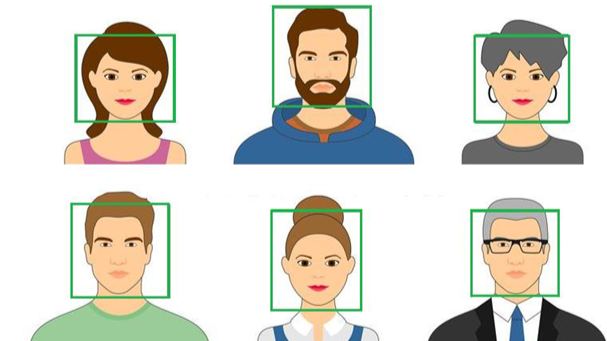
Below given is the example shown in which this classifier was tried. And it detected every face accurately.
References:
Viola, P. and Jones, M. (2001). Rapid Object Detection using a Boosted Cascade of Simple Features. ACCEPTED CONFERENCE ON COMPUTER VISION AND PATTERN RECOGNITION. [online] Available at: https://www.cs.cmu.edu/~efros/courses/LBMV07/Papers/viola-cvpr-01.pdf.
Integral Image | Face Detection. [online] Available at: https://www.youtube.com/watch?v=5ceT8O3k6os&t=198s
Python-for-computer-vision-with-opencv-and-deep-learning Udemy Course. [online] [https://www.udemy.com/course/python-for-computer-vision-with-opencv-and-deep-learning]
Azarcoya-Cabiedes, Willy & Vera-Alfaro, Pablo & Torres-Ruiz, Alfonso & Salas-Rodríguez, Joaquín. (2014). Automatic detection of bumblebees using video analysis. Dyna (Medellin, Colombia). 81. 81–84. 10.15446/dyna.v81n186.40475.
#ArtificialIntelligence #MachineLearning #ComputerVision #DataScience