8 - Performing Simple Linear Regression Using PROC REG in SAS

Simple Linear Regression

Simple linear regression is a statistical method used to model the relationship between two variables by fitting a straight line to the observed data. It estimates how one variable (the dependent variable) changes as the other variable (the independent variable) varies. This technique is commonly used for predictive analysis and determining the strength and direction of relationships between variables.

In order to create your simple linear regression model, you estimate the unknown population parameters β0 and β1. They define the assumed relationship between your response and predictor variable.

Estimate β0 and β1 to determine the line that's as close as possible to all the data points using the method of least squares. This method determines the line that minimizes the sum of the squared vertical distances between the data points and the fitted line. Estimated parameters are denoted with a hat above the parameter, in this case, β0-hat and β1-hat.

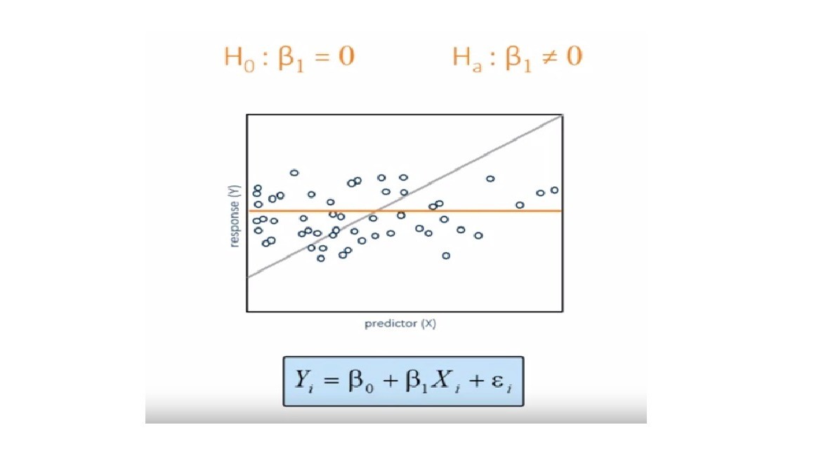
Comparing the Regression Model to a Baseline Model

To determine whether the predictor variable explains a significant amount of variability in the response variable, the simple linear regression model is compared to the baseline model.

The fitted regression line in a baseline model is just a horizontal line across all values of the predictor variable. The slope of this line is 0, and the y-intercept is the sample mean of Y, which is Y-bar.

To determine whether a simple linear regression model is better than the baseline model, you compare the explained variability to the unexplained variability similarly to ANOVA.

In simple linear regression, the variability of the dependent variable Y can be decomposed into three key components:

1 - Explained Variability (Model Sum of Squares - SSM)

This measures the variability in Y that is explained by the linear relationship with X. It represents the part of the total variability that can be explained by the regression model. SSM is the amount of variability that your model explains.

The explained variability is related to the difference between the regression line and the mean of the response variable.

2 - Unexplained Variability (Error Sum of Squares - SSE)

The unexplained variability is the difference between the observed values and the regression line. The amount of variability that our model fails to explain.

3 - Total Variability (SST)

Total variability is the difference between the observed values and the mean of the response variable. It is the sum of model and error sum of squares.

SST = SSM + SSE

• The Sum of Squares for the Model (SSM) and the Sum of Squares for Error (SSE) are divided by their corresponding degrees of freedom to calculate the Mean Square Regression (MSM) and Mean Square Error (MSE).
• The significance of the regression analysis is evaluated similarly to an Analysis of Variance (ANOVA), by computing the F statistic (the ratio of the Mean Square Regression (MSM) to the Mean Square Error (MSE)) and the corresponding p-value. In fact, you'll see an ANOVA table in your regression output as well.

Hypothesis Testing and Assumptions for Linear Regression

Our equation for simple linear regression is this:

So in our hypothesis test we need to chexk the slope β1 is equal to 0 or not.

If the estimated simple linear regression model does not fit the data better than the baseline model, you fail to reject the null hypothesis. Thus, you do not have enough evidence to say that the slope of the regression line in the population differs from zero. If the estimated simple linear regression model does fit the data better than the baseline model, you reject the null hypothesis. Thus, you do have enough evidence to say that the slope of the regression line in the population differs from zero and that the predictor variable explains a significant amount of variability in the response variable.

4 assumptions must be met in order the test to be valid:

1. Mean of the response variable is linearly related to the value of the predictor variable
2. Normally distributed error terms.
3. Error terms have equal variances
4. Error terms are independent at each value of the predictor variable.

The Simple Linear Regression Model

The Simple Linear Regression Model describes the relationship between two variables using a straight line. The model assumes that the dependent variable Y can be expressed as a linear function of the independent variable X. The equation for the model is:

Where:

• Y is the dependent / response variable.
• X is the independent / predictor variable.
• β0 is the intercept (the value of Y when X=0).
• β1 is the slope of the line (the change in Y for a one-unit change in X).
• ε is the error term, representing the difference between the observed and predicted values of Y.

ods graphics;

proc reg data=STAT1.bodyfat2;
    model PctBodyFat2 = Weight ;
    title "Simple Regression with Weight as Regressor";
run;
quit;

title;        

Here is the result, we can buil model equation from the parameter estimates table.

PctBodyFat2 = -12.05 + 0.17 * Weight